Forecast Graveyard

01The result

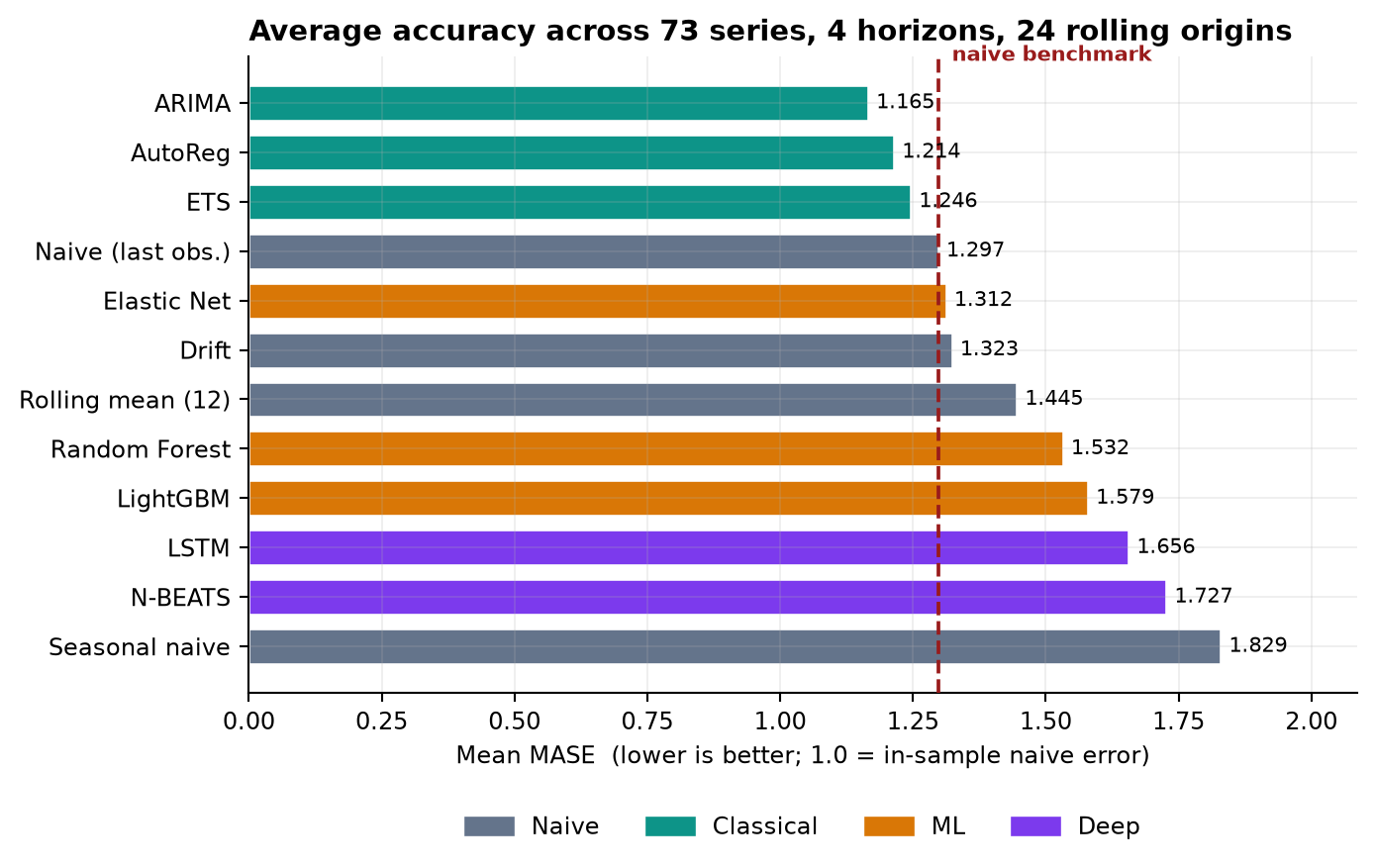
Mean MASE across every series, horizon and origin. MASE is scale-free, so each series counts equally regardless of the units it is measured in. Lower is better; the naive row is the benchmark.

Model	Family	MASE	vs. naive	Win rate
ARIMA ✓	classical	1.165	+10.2%	55.2%
AutoReg ✓	classical	1.214	+6.4%	53.8%
ETS ✓	classical	1.246	+4.0%	53.7%
Naive (last observation)	naive	1.297	+0.0%	50.0%
Elastic Net	ML	1.312	-1.1%	53.9%
Drift	naive	1.323	-2.0%	40.7%
Rolling mean (12)	naive	1.445	-11.4%	49.7%
Random Forest	ML	1.532	-18.1%	48.7%
LightGBM	ML	1.579	-21.7%	48.8%
LSTM	deep	1.656	-27.6%	47.6%
N-BEATS	deep	1.727	-33.1%	47.8%
Seasonal naive	naive	1.829	-41.0%	40.3%

In this benchmark, the classical family was the only one to outperform the naive forecast on aggregate MASE. The machine-learning and deep-learning models did not. 3 of 11 non-naive models improved on it.

After Benjamini–Hochberg FDR control across all 3,212 Diebold–Mariano tests, only 86 beat naive — “no detectable difference” is the verdict for 94% of tests and is the modal outcome for every model.

Mean MASE by model, coloured by family — Mean MASE by model. The dashed line is the naive benchmark; everything to its right lost to a forecast of “next month looks like this month”.

Scope: this is a statement about this universe of 73 univariate monthly US macro series, not about machine learning or deep learning in general.

02The graveyard

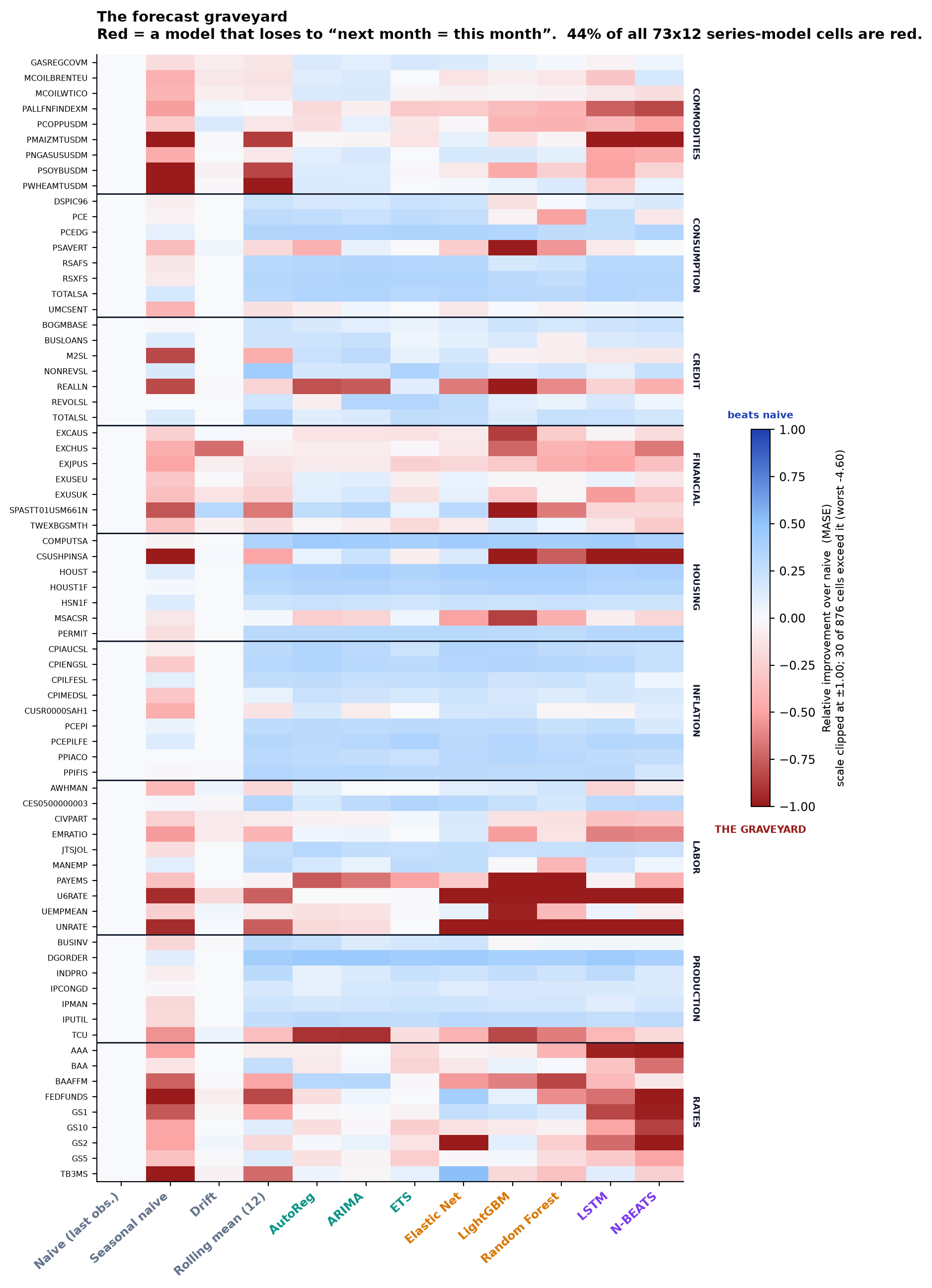
One cell per series and model: the relative reduction in error against the naive forecast. Red is the graveyard.

Series by model heatmap of
relative improvement over the naive forecast — Every red cell is a model that lost to “next month looks like this month”. Series are grouped by category and ordered within each group by how beatable they are.

03The explanation

The ranking is the setup. The question is what determines it — and most of it is decided before a single model is fitted.

21.1%variance in per-series improvement explained by the pre-specified transformation

7.0%explained by the choice of model

The pre-specified transformation explained about 3× as much variation in forecasting improvement as model choice did (η², over 803 series × model cells, naive excluded). Deciding whether you are modelling a near-unit-root level or a growth rate matters more than which model you then reach for.

Transformation	Best model	Mean over models
`diff`	+34.9%	+27.7%
`mom_pct`	+24.3%	+16.1%
`yoy_pct`	+22.5%	-71.8%
`log`	+7.2%	-18.7%
`level`	-1.4%	-29.4%

The naive forecast survives 27% of level-like cells against 19% of growth-rate cells, while deep models win 18% of growth-rate cells against 7% of level-like ones. Near-unit-root targets are where doing nothing is hardest to beat.

Winning model family by series
and horizon, and the same outcomes in meta-feature space — Winning family for each of the 73 × 4 cells, and the same outcomes placed in the two meta-features that separate them best — faceted by horizon, because meta-features are per-series and a single scatter would hide three of every four points.

04What the complexity costs

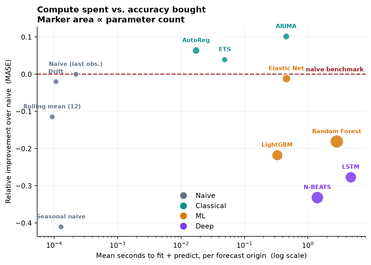
Model	Slower than naive	vs. naive	Peak RAM
Naive (last observation)	1×	+0.0%	-0 MB
ARIMA	2,069×	+10.2%	34 MB
Elastic Net	2,093×	-1.1%	22 MB
LightGBM	1,491×	-21.7%	29 MB
Random Forest	13,017×	-18.1%	47 MB
LSTM	21,612×	-27.6%	255 MB
N-BEATS	6,422×	-33.1%	235 MB

The LSTM is 21,612× slower than a naive forecast and 28% worse. Peak memory is measured by fitting each model in a fresh subprocess, minus a baseline child that imports the same libraries and fits nothing.

Compute spent against
accuracy bought, by model — Compute spent against accuracy bought. Marker area is proportional to parameter count; the horizontal axis is log-scaled.

05A metric that inverts the answer

Methodological trap

Averaging raw absolute errors across the registry says 10 of 11 non-naive models beat the naive forecast — roughly 33% better each, and very nearly the opposite conclusion to the one above.

That aggregate is dominated by a handful of high-scale series. Housing starts are seasonally-adjusted annual counts in the hundreds; CPI inflation is a fraction of a percent per month. Three housing series alone contribute about 70% of the registry's pooled MAE, so a pooled-MAE improvement is close to a statement about housing starts rather than about 73 series.

Pooled MAE is kept in the report only as a cautionary comparison. Every headline number here uses the scale-free metric.

06Can the winner be predicted in advance?

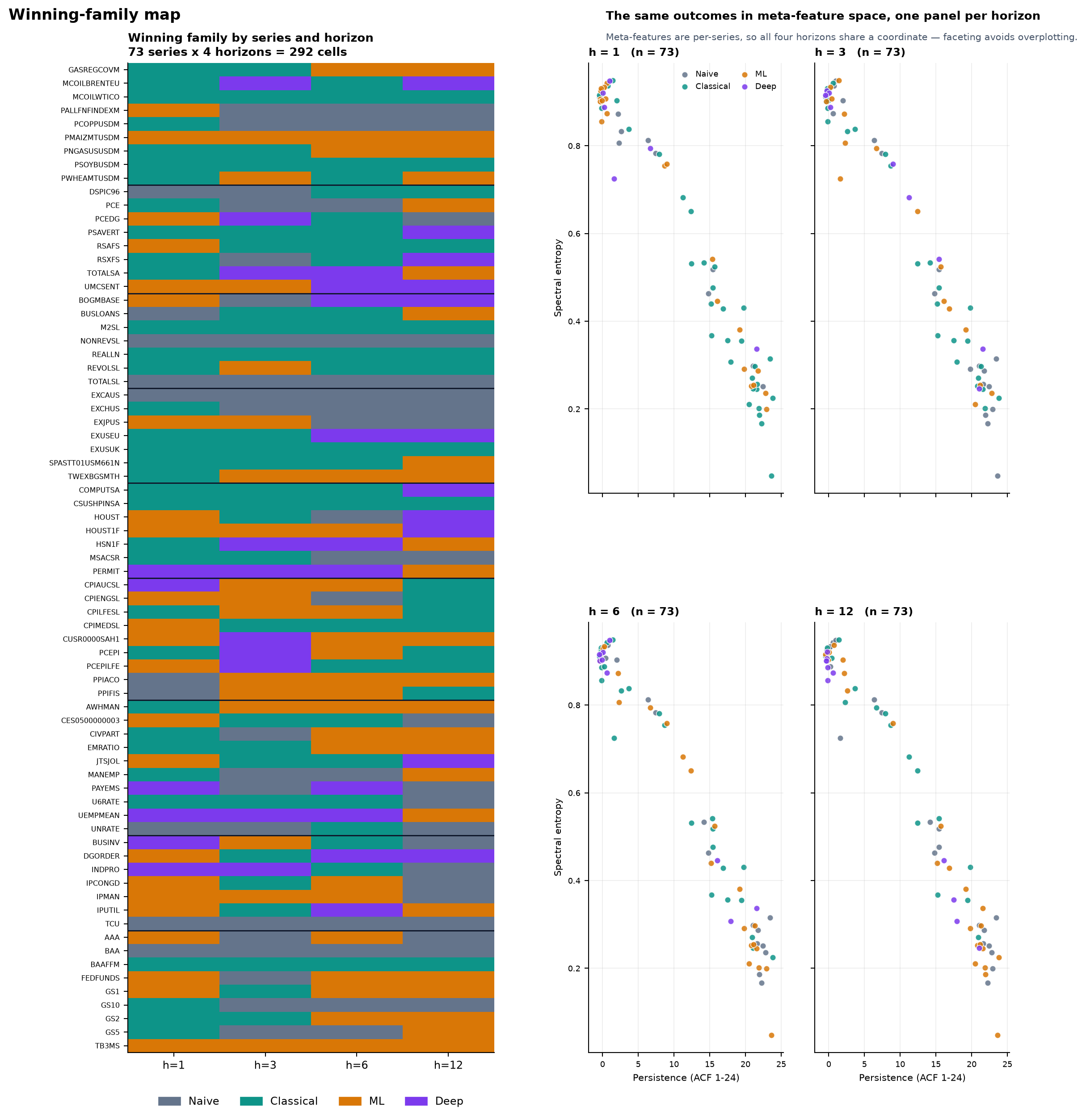
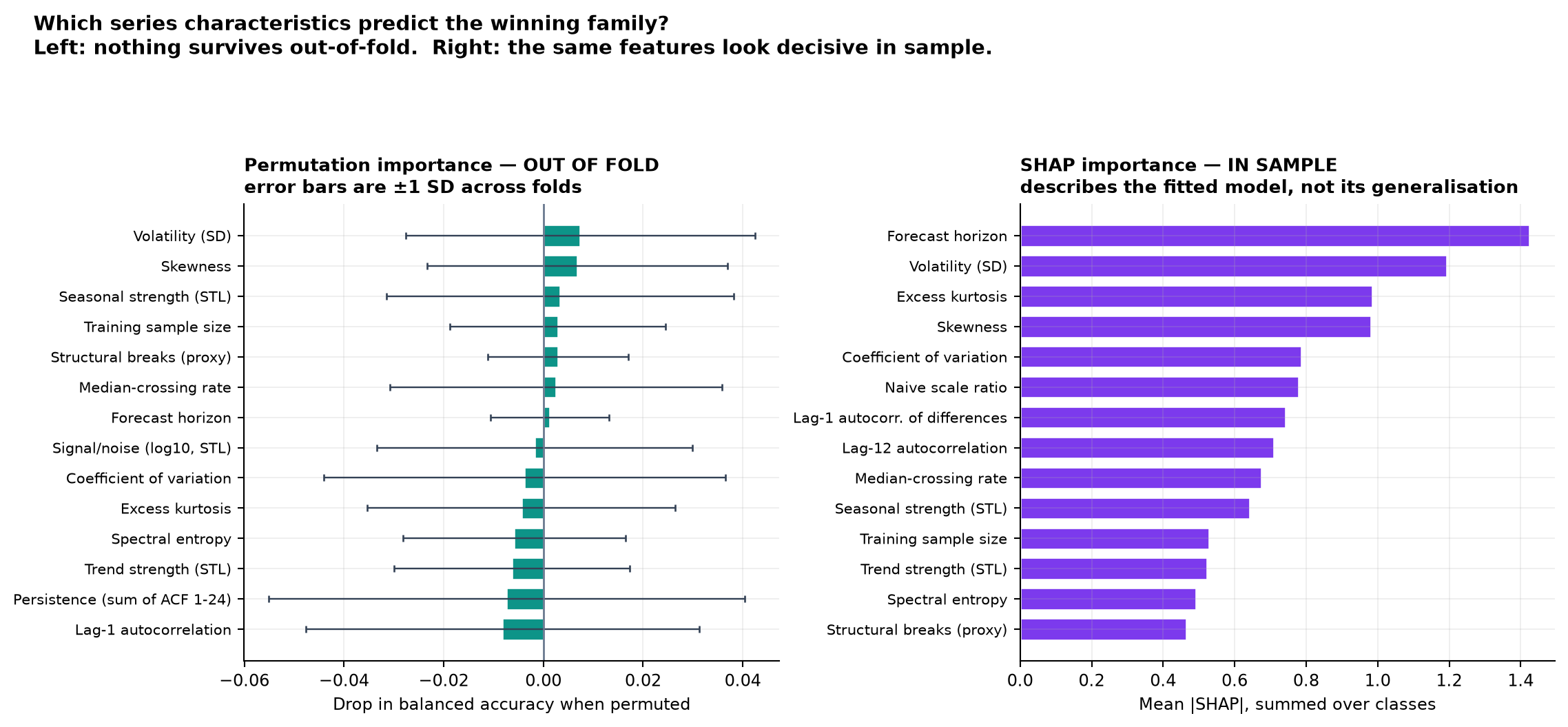
A meta-model predicts the winning family for each series and horizon from characteristics computable before any forecast is made. Validation holds out whole series, so all four horizons of a series are unseen together.

0.375balanced accuracy, leave-series-out (random_forest)

0.250majority-class baseline

Real, but modest. The marginal associations are strong and readable — yet no single feature's out-of-fold permutation importance exceeds twice its own standard deviation across folds. Individually informative features do not compose into a rule that transfers to an unseen series.

Out-of-fold permutation importance
beside in-sample SHAP importance for the meta-model — Left: nothing survives out of fold. Right: the same features look decisive in sample. The contrast is the finding.

07Limitations

Univariate only. No exogenous regressors and no cross-series information. Much of machine learning's value in macro forecasting comes from wide panels; this study deliberately isolates the univariate case.
Current vintages, not real-time vintages, so revisions are ignored. Revisions would make every model's job harder and would penalise models that lean hardest on the most recent observation.
The recession/expansion split is not estimable and is not reported. The evaluation window (2023-08 to 2026-08) lies entirely within an NBER-dated expansion: the expansion bucket holds 83,616 scored forecasts and the recession bucket holds 0. The machinery is implemented and tested; the data window does not support the claim.
24 origins per series is a realistic amount of monthly macro data and is thin for statistical power. The Diebold–Mariano results mean “cannot distinguish”, not “identical”.
A fixed hyper-parameter budget by design. A per-series search would change the accuracy numbers and make the compute comparison meaningless.
One seed per model. The deep models are bit-reproducible, but their across-seed variability is not characterised here.

08Method & reproducibility

Expanding-window rolling origin. 24 origins per series, every model refit from scratch at every origin. No random splits anywhere.
Transformations pre-registered from each series' economic type and never revised in response to accuracy.
MASE scaled by the mean absolute one-step naive error on the first training window — constant per series and observable at every origin.
Diebold–Mariano with a Newey–West variance truncated at h−1 and the Harvey–Leybourne–Newbold correction, then Benjamini–Hochberg FDR across the whole family of tests.
Every individual forecast is stored — prediction, actual, both errors, runtime, parameter count and seed — so any number above can be traced back to the forecasts that produced it.

Data comes from FRED's public CSV endpoint; no API key is required.

git clone https://github.com/Gariyuuu/forecast-graveyard.git
uv venv --python 3.12 .venv
uv pip install --python .venv/bin/python -e ".[dev]"

python scripts/run_study.py backtest   # ~15 CPU-hours, resumable
python scripts/run_study.py analyse    # tables, meta-model, figures, report

pytest -q                              # test suite
python scripts/verify_artifacts.py     # documented claims vs. artifacts

Every number on this page is read out of the stored result files at build time. The build fails if a referenced table or figure is missing.